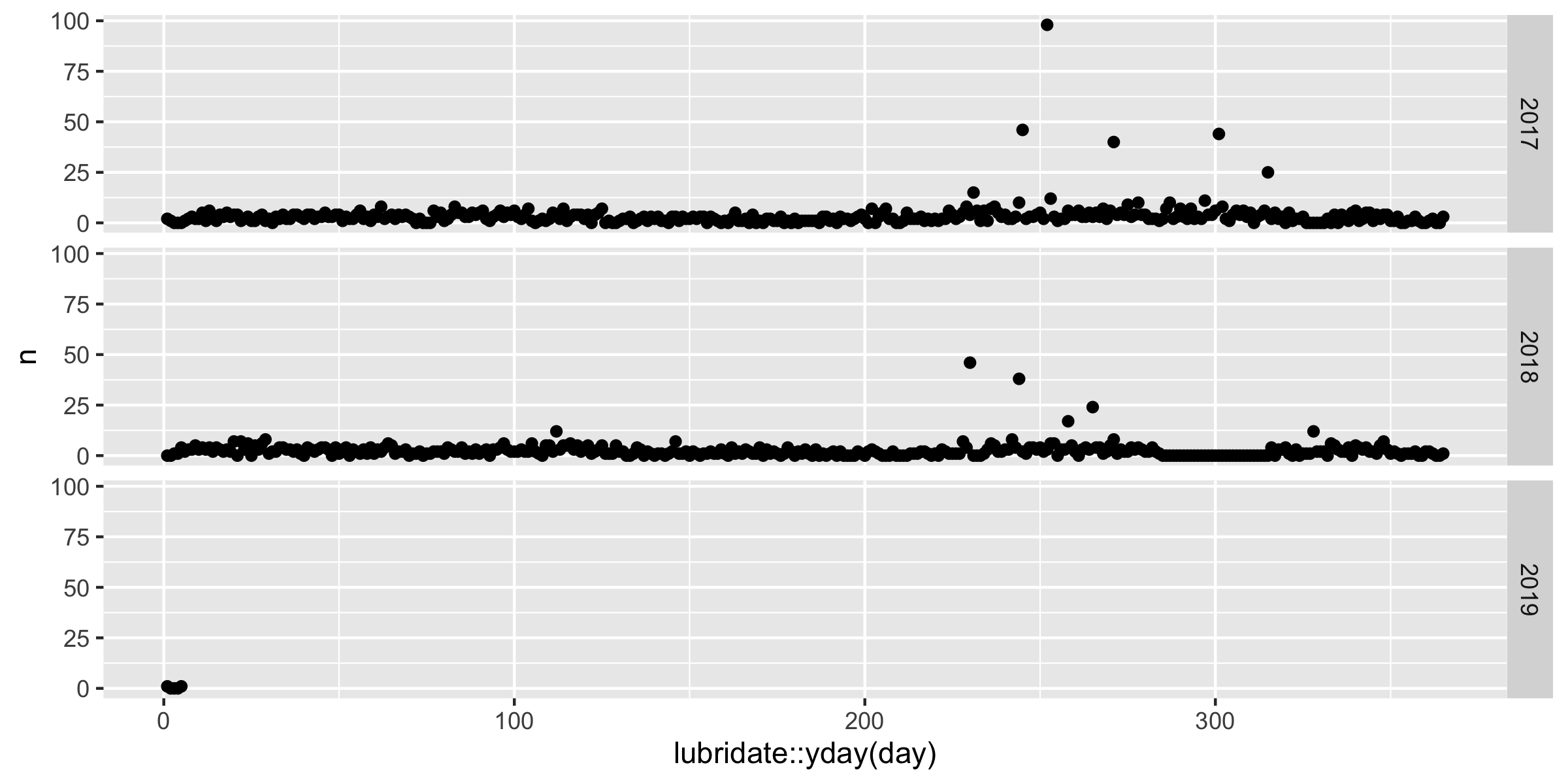
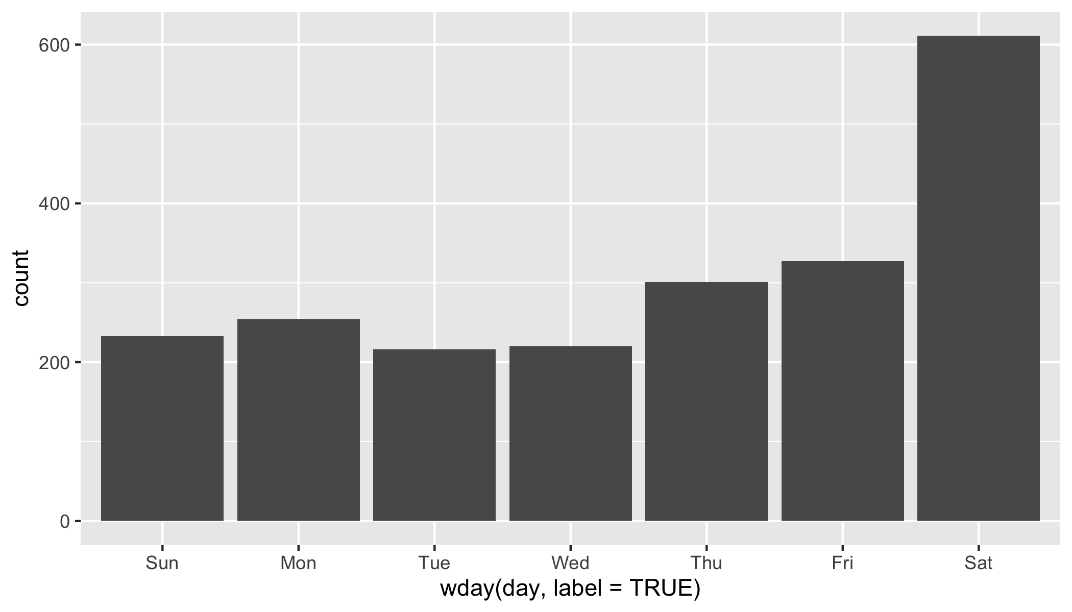
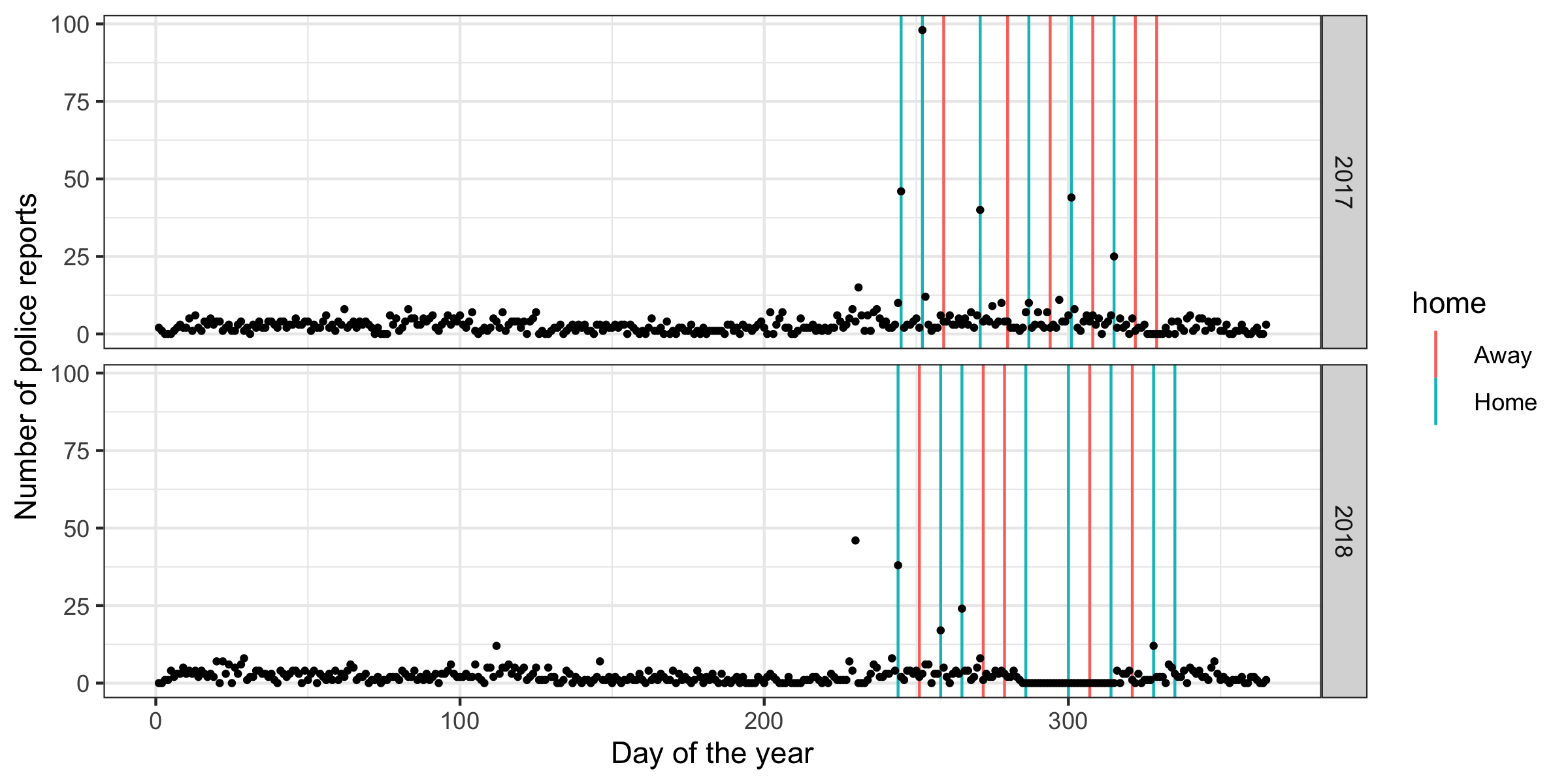
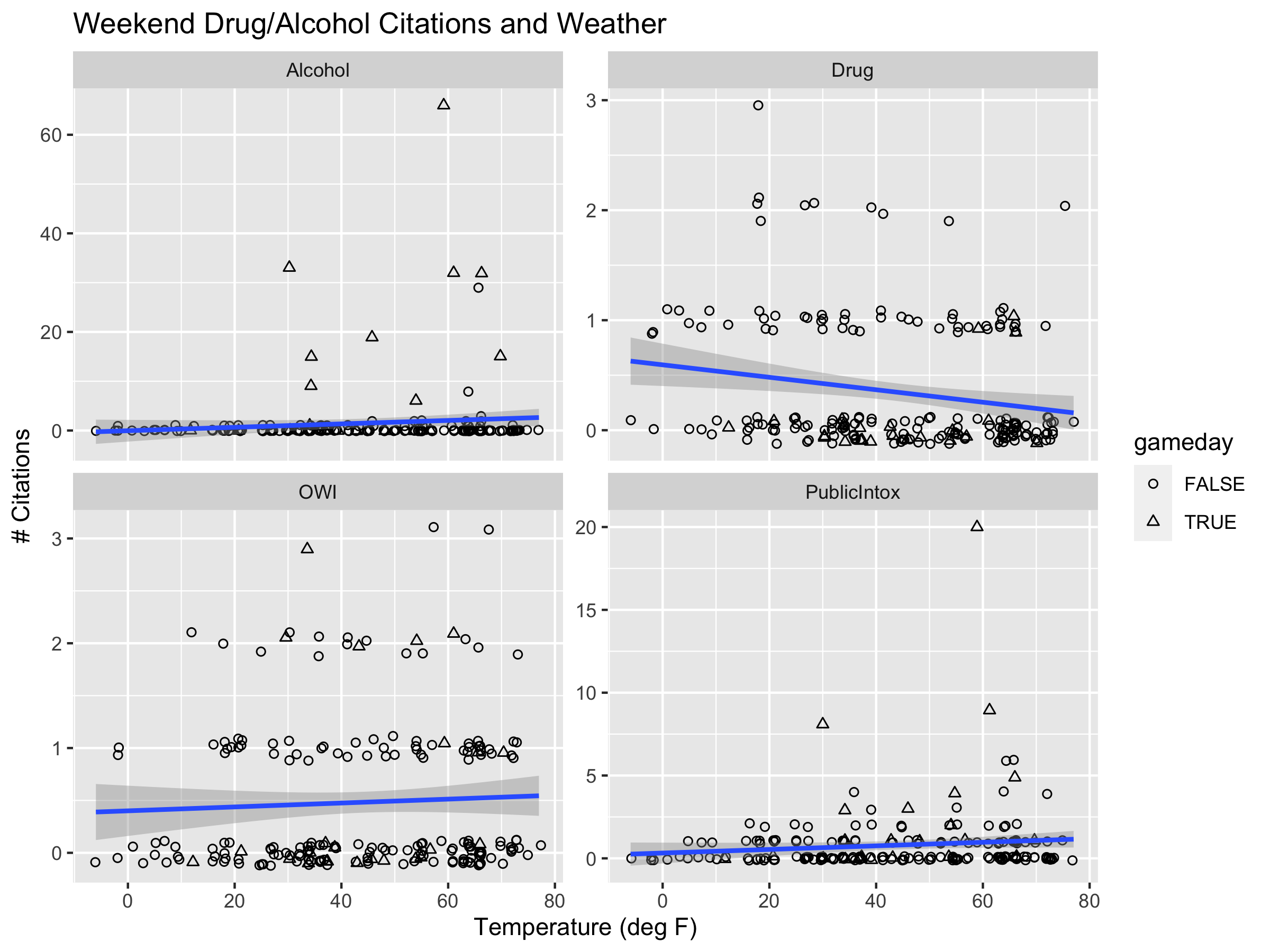
class: center, middle, inverse, title-slide .title[ # Stat 585 - elements of the tidyverse ] .author[ ### Heike Hofmann ] --- ## tidyverse `tidyverse` is an 'opinionated' package bundling several other R packages for data science tasks: ```r tidyverse::tidyverse_packages() ``` ``` ## [1] "broom" "cli" "crayon" "dbplyr" ## [5] "dplyr" "dtplyr" "forcats" "ggplot2" ## [9] "googledrive" "googlesheets4" "haven" "hms" ## [13] "httr" "jsonlite" "lubridate" "magrittr" ## [17] "modelr" "pillar" "purrr" "readr" ## [21] "readxl" "reprex" "rlang" "rstudioapi" ## [25] "rvest" "stringr" "tibble" "tidyr" ## [29] "xml2" "tidyverse" ``` - https://cran.r-project.org/web/packages/tidyverse/vignettes/manifesto.html - share common data representations and API, i.e. work well together - see https://github.com/hadley/tidyverse for more information: [R for Data Science](https://r4ds.had.co.nz/) - run `tidyverse::tidyverse_update()` to check if/which for updates --- ## Graphical and numerical summaries 1. graphical summaries - visualizations with `ggplot2`: - [RStudio cheatsheet for ggplot2](hhttps://raw.githubusercontent.com/rstudio/cheatsheets/main/data-visualization.pdf) - online documentation: https://ggplot2.tidyverse.org/ - Google group: https://groups.google.com/forum/#!forum/ggplot2 2. numerical summaries - elements of `dplyr` and `tidyr` - assessing data quality; data wrangling - [RStudio cheatsheet for dplyr](https://raw.githubusercontent.com/rstudio/cheatsheets/main/data-transformation.pdf) - [RStudio cheatsheet for tidyr](https://raw.githubusercontent.com/rstudio/cheatsheets/main/tidyr.pdf) --- ## The pipe operator `%>%` `f(x) %>% g(y)` is equivalent to `g(f(x), y)` i.e. the output of one function is used as input to the next function. This function can be the identity Consequences: - `x %>% f(y)` is the same as `f(x, y)` - statements of the form `k(h(g(f(x, y), z), u), v, w)` become `x %>% f(y) %>% g(z) %>% h(u) %>% k(v, w)` - read `%>%` as "then do" --- ## dplyr There are five primary `dplyr` *verbs*, representing distinct data analysis tasks: - **Filter**: Select specified rows of a data frame, produce subsets - **Arrange**: Reorder the rows of a data frame - **Select**: Select particular columns of a data frame - **Mutate**: Add new or change existing columns of the data frame (as functions of existing columns) - **Summarise**: Create collapsed summaries of a data frame - (**Group By**: Introduce structure to a data frame) <br> `dplyr` resources: - https://dplyr.tidyverse.org/ - R for Data Science book: https://r4ds.had.co.nz/transform.html --- class: inverse ## Your Turn The Iowa State Police Department publishes a Daily Crime Log at https://www.police.iastate.edu/crime-log/ Data for 2017 and most of 2018 are available as file [pd-isu.csv](https://raw.githubusercontent.com/Stat585-at-ISU/materials-2023/master/data/isu-pd.csv) from the course website. Read the data into your R session and answer the following questions: - which types of crimes (`Classification`) are typically committed? How many different classifications are there? - which days are in the top ten for 2018? (Use the `lubridate` package to get to date variables) - how many times a day are crimes typically reported? - what else do you find? --- class: middle, center ## <img src = "https://imgs.xkcd.com/comics/tasks_2x.png" height = 300> Don't peek unless you have tried for yourself! --- # a solution ```r library(tidyverse) pd <- read_csv("../data/isu-pd.csv") pd %>% count(Classification) %>% dim() ``` ``` ## [1] 147 2 ``` ```r # 147 different types of crime classifications pd %>% count(Classification, sort = TRUE) %>% head() ``` ``` ## # A tibble: 6 × 2 ## Classification n ## <chr> <int> ## 1 Theft 400 ## 2 Alcohol Violation 341 ## 3 Public Intoxication 245 ## 4 Drug Violation 231 ## 5 Operating while Intoxicated 145 ## 6 Harassment 124 ``` --- Let's check the back, too ```r pd %>% count(Classification, sort = TRUE) %>% tail() ``` ``` ## # A tibble: 6 × 2 ## Classification n ## <chr> <int> ## 1 Trespass 1 ## 2 Vandalism / Disorderly Conduct 1 ## 3 Vandalism / Public Intoxication 1 ## 4 Vandalism / Trespass 1 ## 5 Vandalism/Disorderly Conduct/Criminal Trespass 1 ## 6 Weapons Violation 1 ``` --- # break multiple citings into Main and rest ```r pd <- pd %>% separate(Classification, into = "Main", sep="/", remove = FALSE) %>% mutate( Main = trimws(Main) ) pd %>% count(Main, sort = TRUE) %>% head() ``` ``` ## # A tibble: 6 × 2 ## Main n ## <chr> <int> ## 1 Theft 401 ## 2 Alcohol Violation 353 ## 3 Public Intoxication 281 ## 4 Drug Violation 279 ## 5 Operating while Intoxicated 179 ## 6 Harassment 125 ``` doesn't change much --- ## Top ten bad days in 2018 first get dates, see [RStudio lubridate cheat sheet](https://github.com/rstudio/cheatsheets/raw/master/lubridate.pdf): ```r library(lubridate) head(pd$`Date/Time Reported`) ``` ``` ## [1] "01/01/17 1643" "01/01/17 2107" "01/02/17 0257" "01/06/17 1358" ## [5] "01/07/17 0107" "01/07/17 2131" ``` ```r pd$date <- lubridate::mdy_hm(pd$`Date/Time Reported`) summary(pd$date) ``` ``` ## Min. 1st Qu. ## "2017-01-01 16:43:00.0000" "2017-08-08 05:39:00.0000" ## Median Mean ## "2017-10-28 12:47:30.0000" "2017-12-07 17:29:53.1729" ## 3rd Qu. Max. ## "2018-05-04 11:09:00.0000" "2019-01-05 22:12:00.0000" ``` --- ## Top ten bad days in 2018 (2) Now we want to just have the day rather than the time ```r pd$day <- lubridate::as_date(pd$date) head(pd$day) ``` ``` ## [1] "2017-01-01" "2017-01-01" "2017-01-02" "2017-01-06" "2017-01-07" ## [6] "2017-01-07" ``` --- ## Top ten bad days in 2018 (3) ```r pd %>% count(day, sort = TRUE) %>% filter(lubridate::year(day) == 2018) %>% head(10) ``` ``` ## # A tibble: 10 × 2 ## day n ## <date> <int> ## 1 2018-08-18 46 ## 2 2018-09-01 38 ## 3 2018-09-22 24 ## 4 2018-09-15 17 ## 5 2018-04-22 12 ## 6 2018-11-24 12 ## 7 2018-01-29 8 ## 8 2018-08-30 8 ## 9 2018-09-28 8 ## 10 2018-01-20 7 ``` --- ## Average number of reports per day Why is this average not right for the average number of reports by day? ```r pd %>% count(day) %>% summary() ``` ``` ## day n ## Min. :2017-01-01 Min. : 1.000 ## 1st Qu.:2017-06-20 1st Qu.: 2.000 ## Median :2017-12-06 Median : 3.000 ## Mean :2017-12-12 Mean : 3.603 ## 3rd Qu.:2018-05-27 3rd Qu.: 4.000 ## Max. :2019-01-05 Max. :98.000 ``` -- Problem: we are missing days with zero reports. --- class: inverse ## Your Turn We want to find an elegant solution to the zero reports a day problem. The function `complete` in the `tidyr` package looks promising. Try to get it to work for this problem. --- class: middle, center ## ... only after you tried ... --- ## Average number of reports per day (2) Why is this still wrong? ```r pd %>% complete(day = full_seq(pd$day, period = 1)) %>% count(day) %>% summary() ``` ``` ## day n ## Min. :2017-01-01 Min. : 1.000 ## 1st Qu.:2017-07-03 1st Qu.: 1.000 ## Median :2018-01-03 Median : 2.000 ## Mean :2018-01-03 Mean : 3.125 ## 3rd Qu.:2018-07-05 3rd Qu.: 4.000 ## Max. :2019-01-05 Max. :98.000 ``` --- ## Average number of reports per day (2) What does `complete` do exactly? ```r pd %>% complete(day = full_seq(pd$day, period = 1)) ``` ``` ## # A tibble: 2,297 × 10 ## day Case Numbe…¹ Class…² Main Date/…³ Earli…⁴ Lates…⁵ Gener…⁶ Dispo…⁷ ## <date> <chr> <chr> <chr> <chr> <chr> <chr> <chr> <chr> ## 1 2017-01-01 17-000001 Drug V… Drug… 01/01/… 01/01/… 01/01/… 124 Un… Arrest ## 2 2017-01-01 17-000002 Drug V… Drug… 01/01/… 01/01/… 01/01/… Foutai… Arrest ## 3 2017-01-02 17-000003 Drug V… Drug… 01/02/… 01/02/… 01/02/… Lincol… Arrest ## 4 2017-01-03 <NA> <NA> <NA> <NA> <NA> <NA> <NA> <NA> ## 5 2017-01-04 <NA> <NA> <NA> <NA> <NA> <NA> <NA> <NA> ## 6 2017-01-05 <NA> <NA> <NA> <NA> <NA> <NA> <NA> <NA> ## 7 2017-01-06 17-000008 Drug V… Drug… 01/06/… <NA> 01/06/… Armory… Open ## 8 2017-01-07 17-000010 Public… Publ… 01/07/… 01/07/… 01/07/… 204 We… Arrest ## 9 2017-01-07 17-000011 Alcoho… Alco… 01/07/… 01/07/… 01/07/… 119 St… Arrest ## 10 2017-01-08 17-000012 Drug V… Drug… 01/08/… 01/08/… 01/08/… Hawtho… Arrest ## # … with 2,287 more rows, 1 more variable: date <dttm>, and abbreviated ## # variable names ¹​`Case Number`, ²​Classification, ³​`Date/Time Reported`, ## # ⁴​`Earliest Occurrence`, ⁵​`Latest Occurrence`, ⁶​`General Location`, ## # ⁷​Disposition ``` --- ## Average number of reports per day (3) ```r perday <- pd %>% complete(day = full_seq(pd$day, period = 1)) %>% group_by(day) %>% summarize( n = sum(!is.na(Classification)) ) perday %>% summary() ``` ``` ## day n ## Min. :2017-01-01 Min. : 0.000 ## 1st Qu.:2017-07-03 1st Qu.: 1.000 ## Median :2018-01-03 Median : 2.000 ## Mean :2018-01-03 Mean : 2.942 ## 3rd Qu.:2018-07-05 3rd Qu.: 4.000 ## Max. :2019-01-05 Max. :98.000 ``` --- ## Crime reports over time ```r perday %>% mutate(year = lubridate::year(day)) %>% ggplot(aes( x = lubridate::yday(day), y = n)) + geom_point() + facet_grid(year~.) ``` <!-- --> --- # ... it's the Saturdays that are tricky ```r perday %>% ggplot(aes(x = wday(day, label =TRUE), weight = n)) + geom_bar() ``` <!-- --> --- class: inverse ## Your turn The files [isu-football-2017.csv](https://raw.githubusercontent.com/Stat585-at-ISU/materials-2023/master/data/isu-football-2017.csv) and [isu-football-2018.csv](https://raw.githubusercontent.com/Stat585-at-ISU/materials-2023/master/data/isu-football-2018.csv) consist of the Cyclones' football schedule in 2017 and 2018. Use the data to create the chart below: <!-- --> Don't forget to *look at* the chart. What are your main findings? --- ```r # read in schedules and clean up dates schedule <- read.csv("../data/isu-football-2018.csv") schedule <- schedule %>% mutate( date = lubridate::ymd("2018-01-01") ) lubridate::month(schedule$date) <- as.numeric(factor(schedule$Month, levels=c("Sep", "Oct", "Nov", "Dec"))) + 8 lubridate::mday(schedule$date) <- schedule$Day schedule$yday <- lubridate::yday(schedule$date) schedule$year <- lubridate::year(schedule$date) schedule17 <- read.csv("../data/isu-football-2017.csv") schedule17 <- schedule17 %>% mutate( date = lubridate::mdy(Date) ) schedule17$yday <- lubridate::yday(schedule17$date) schedule17$year <- lubridate::year(schedule17$date) ``` --- ```r perday %>% mutate( year = lubridate::year(day), yday = lubridate::yday(day) ) %>% filter(year <= 2018) %>% ggplot(aes(x = yday, y = n)) + geom_vline(data = schedule, aes(xintercept = yday, colour = home)) + geom_vline(data = schedule17, aes(xintercept = yday, colour = Home)) + geom_point(size = .75) + facet_grid(year~.) + theme_bw() + ylab("Number of police reports") + xlab("Day of the year") ``` <!-- --> --- # Strange findings <!-- --> - one large outlier not related to football games in Ames - one game at home not resulting in large number of crime logs? (Kansas - ISU 0 - 45) - range of two weeks in October 2018 with no crimes logged --- ## Tools for working with data - moving between wide and long forms of data: - `pivot_longer` (formerly `gather`) - `pivot_wider` (formerly `spread`) - see https://r4ds.had.co.nz/tidy-data.html - joining data sets: `left_join`, `anti_join`, see also https://r4ds.had.co.nz/relational-data.html --- class: inverse ## Your turn Does the weather affect the number of citations for drug and alcohol-related offenses? Use [Ames_weather_2017-2018.csv](https://raw.githubusercontent.com/Stat585-at-ISU/materials-2023/master/data/Ames_weather_2017-2018.csv) and combine the data with relevant Ames PD data. Graphically examine the relationship between temperature and number of citations. You may find it helpful to only consider Thursday - Saturday. ```r ames_weather <- read_csv("../data/Ames_weather_2017-2018.csv") %>% filter(!is.na(time)) # summarize by day to get daily highs and lows ames_weather_daily <- ames_weather %>% mutate(day = as.Date(date)) %>% group_by(day) %>% summarize(temp_low = min(temp_low), temp_high = max(temp_high)) ``` .small[For the curious: [script to get the weather data](https://gist.github.com/srvanderplas/9f4a471e0fb19495935fb2104f3ba9f8)] --- class: middle,center ... only after you tried ... --- ```r library(lubridate) substitutions <- c("P[uU]blic Intox.*" = "PublicIntox", "Drug Violation" = "Drug", "Alcohol Violation" = "Alcohol", "Operating [wW]hile Intoxicated" = "OWI") # Get relevant Ames PD data drug_alcohol_daily <- pd %>% filter(str_detect(Main, "Alcohol|Drug|Intox")) %>% mutate(Main = str_replace_all(Main, substitutions)) %>% mutate(day = floor_date(date, unit = "day") %>% as.Date()) %>% group_by(Main, day) %>% summarize(n = n()) %>% complete(day = full_seq(.$day, period = 1), fill = list(n = 0)) ``` ``` ## `summarise()` has grouped output by 'Main'. You can override using the ## `.groups` argument. ``` --- ```r game_days <- unique(c(schedule$date, schedule17$date)) # Combine the data with weather data wkd_weather_cites <- drug_alcohol_daily %>% left_join(ames_weather_daily) %>% mutate(wday = wday(day, label = T)) %>% # Show game days mutate(gameday = day %in% game_days) %>% filter(wday %in% c("Thurs", "Fri", "Sat")) ``` ``` ## Joining, by = "day" ``` ```r # Plot wkd_weather_cites %>% ggplot(aes(x = temp_low, y = n)) + # Jitter in y a bit so points don't overlap as much geom_jitter(aes(shape = gameday), height = .125) + geom_smooth(aes(x = temp_low, y = n), method = "lm") + facet_wrap(~Main, scales = "free_y") + scale_shape_manual(values = c(1, 2)) + ggtitle("Weekend Drug/Alcohol Citations and Weather") + scale_x_continuous("Temperature (deg F)") + scale_y_continuous("# Citations") ``` ``` ## `geom_smooth()` using formula = 'y ~ x' ``` --- class:center  --- # Adding to the data The ISU-PD department still posts the crime log - but now, in form of a pdf of what looks like a spread sheet. Can we still get usable data out of this format? -- There is a package `pdftools` available on CRAN ... but it does not return a data frame (or a tibble) as result. We need to look at other formats that R offers ..