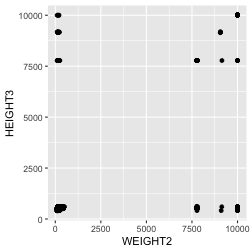
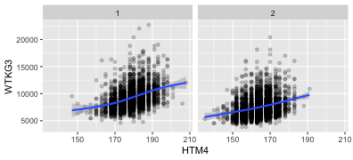
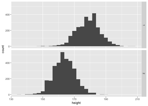
class: center, middle, inverse, title-slide .title[ # Stat 585 - Working in teams: Sample solution for the test case ] .author[ ### Heike Hofmann ] --- class: center, middle # A 'Solution' to the test case --- class: inverse ## A Plan of work 0. Find out where the data comes from 1. Describe the working environment 2. Verify that there are variables for height and weight in the data and read the description of the variables in the codebook. 3. Calculate averages for height and weight, then report. 4. Calculate correlation between height and weight, then report. 5. Write a short report of your findings. Address potential problems in the data. --- # A solution attempt 0. Setup - this solution uses R v4.2.2 in RStudio (2022.12.0 Build 352). - You need the R packages `tidyverse` and `rmarkdown` to run the solution - use the command `install.packages(c("tidyverse","rmarkdown"))` in the R console to install the two packages 1. Navigate to https://github.com/Stat585-at-ISU/materials-2023 2. Download the file [`test-case-solution.Rmd`](https://raw.githubusercontent.com/Stat585-at-ISU/materials-2023/master/01_collaborative-environment/test-case-solution.Rmd) in folder `01_collaborative-environment` in RStudio to get this set of slides. 3. "Knit" the file (Click on the button in the menu). --- ## The Data Source The dataset `brfss_iowa.csv` (linked from website) contains 6227 records from the Behavioral Risk Factor Surveillance System (BRFSS) for Iowans. > The Behavioral Risk Factor Surveillance System (BRFSS) is the nation's premier system of health-related telephone surveys that collect state data about U.S. residents regarding their health-related risk behaviors. It is conducted annually by the Center for Disease Control and Prevention (CDC). Codebook with detailed explanations of variables is [available here](https://www.cdc.gov/brfss/annual_data/2015/pdf/codebook15_llcp.pdf). --- ## What is the relationship between height and weight? Read the data: ```r library(tidyverse) iowa <- readr::read_csv("https://github.com/Stat585-at-ISU/materials/raw/master/01_collaborative-environment/data/brfss_iowa.csv") # the read_csv function from the readr package is faster than the standard read.csv # but the output is a tibble (we'll come back to that) iowa ``` ``` ## # A tibble: 6,227 × 330 ## X_STATE FMONTH IDATE IMONTH IDAY IYEAR DISPC…¹ SEQNO X_PSU CTELE…² PVTRE…³ ## <dbl> <dbl> <chr> <chr> <chr> <dbl> <dbl> <dbl> <dbl> <dbl> <dbl> ## 1 19 7 0708… 07 08 2015 1200 2.02e9 2.02e9 NA NA ## 2 19 3 0321… 03 21 2015 1200 2.02e9 2.02e9 NA NA ## 3 19 10 0110… 01 10 2016 1200 2.02e9 2.02e9 NA NA ## 4 19 4 0509… 05 09 2015 1200 2.02e9 2.02e9 NA NA ## 5 19 5 0624… 06 24 2015 1200 2.02e9 2.02e9 NA NA ## 6 19 7 0803… 08 03 2015 1200 2.02e9 2.02e9 NA NA ## 7 19 7 0812… 08 12 2015 1200 2.02e9 2.02e9 NA NA ## 8 19 7 0810… 08 10 2015 1200 2.02e9 2.02e9 NA NA ## 9 19 10 1115… 11 15 2015 1200 2.02e9 2.02e9 NA NA ## 10 19 8 0813… 08 13 2015 1200 2.02e9 2.02e9 NA NA ## # … with 6,217 more rows, 319 more variables: COLGHOUS <lgl>, STATERES <dbl>, ## # CELLFON3 <dbl>, LADULT <lgl>, NUMADULT <dbl>, NUMMEN <dbl>, NUMWOMEN <dbl>, ## # CTELNUM1 <dbl>, CELLFON2 <dbl>, CADULT <dbl>, PVTRESD2 <dbl>, ## # CCLGHOUS <dbl>, CSTATE <dbl>, LANDLINE <dbl>, HHADULT <dbl>, GENHLTH <dbl>, ## # PHYSHLTH <dbl>, MENTHLTH <dbl>, POORHLTH <dbl>, HLTHPLN1 <dbl>, ## # PERSDOC2 <dbl>, MEDCOST <dbl>, CHECKUP1 <dbl>, BPHIGH4 <dbl>, BPMEDS <dbl>, ## # BLOODCHO <dbl>, CHOLCHK <dbl>, TOLDHI2 <dbl>, CVDINFR4 <dbl>, … ``` --- ## Variables for height and weight ```r grep("HEIGHT", names(iowa), value=TRUE) ``` ``` ## [1] "HEIGHT3" ``` ```r grep("WEIGHT", names(iowa), value=TRUE) ``` ``` ## [1] "WEIGHT2" ``` ```r iowa %>% select(HEIGHT3, WEIGHT2) %>% head() ``` ``` ## # A tibble: 6 × 2 ## HEIGHT3 WEIGHT2 ## <dbl> <dbl> ## 1 511 191 ## 2 7777 140 ## 3 503 135 ## 4 504 115 ## 5 NA NA ## 6 510 210 ``` Variables are there ... but ... some data values look odd. --- ## Codebook excerpt From the [codebook](https://www.cdc.gov/brfss/annual_data/2015/pdf/codebook15_llcp.pdf): HEIGHT3 and WEIGHT2 are the originally recorded variables. <img src="https://github.com/Stat585-at-ISU/materials/raw/master/01_collaborative-environment/images/codebook-height3.png" width=750> Let's plot that ... --- ## Plot Load the `ggplot2` package to plot weight versus height: ```r iowa %>% ggplot(aes(x = WEIGHT2, y = HEIGHT3)) + geom_point() ``` <!-- --> Height and weight should show a somewhat positive correlation. These clusters are an indication of the data coding. --- ## Next steps Obviously, we need to spend some time cleaning these variables before we can make use of them. We have a couple of choices: 1. We can buckle down and do that clean-up and then move on to the calculation. 2. We can take another look at the variables and investigate what `HTIN4`, `HTM4`, and `WTKG3` are ... --- ## Route 2 Let's take the second route first and draw a picture of height and weight in metric units: ```r iowa %>% ggplot(aes(x = HTM4, y = WTKG3)) + geom_point(alpha = 0.2) + facet_grid(.~SEX) + geom_smooth() ``` <!-- --> These charts look much better! We see a general increase in weight as height increases. The variability in weight is huge, though. On average, women (`SEX = 2`) are shorter and lighter. --- ## Look at the variables' values Based on variables `HTM4` and `WTKG3` ```r summary(iowa$HTM4) ``` ``` ## Min. 1st Qu. Median Mean 3rd Qu. Max. NA's ## 135.0 163.0 170.0 170.5 178.0 208.0 232 ``` ```r summary(iowa$WTKG3) ``` ``` ## Min. 1st Qu. Median Mean 3rd Qu. Max. NA's ## 3856 6804 8119 8319 9525 22680 552 ``` -- Height is reported in cm. Weight is reported in tens of grams. --- ## Get results and adjust the units ```r iowa %>% group_by(SEX) %>% summarize( n = n(), avg_height_cm = mean(HTM4, na.rm=TRUE), avg_weight_kg = mean(WTKG3, na.rm=TRUE)/100, cor = cor(HTM4, WTKG3, use="pairwise.complete"), avg_height_in = mean(HTIN4, na.rm=TRUE), non_missing = sum(!is.na(HTM4) & !is.na(WTKG3)), non_missing_perc = non_missing/n*100 ) ``` ``` ## # A tibble: 2 × 8 ## SEX n avg_height_cm avg_weight_kg cor avg_height_in non_miss…¹ non_m…² ## <dbl> <int> <dbl> <dbl> <dbl> <dbl> <int> <dbl> ## 1 1 2704 179. 93.1 0.398 70.5 2589 95.7 ## 2 2 3523 164. 74.8 0.275 64.5 3051 86.6 ## # … with abbreviated variable names ¹​non_missing, ²​non_missing_perc ``` --- ## Route 1 This is quite a bit more work. Don't do things this way! ```r # first of all, replace all missing values by NAs iowa <- iowa %>% mutate( HEIGHT3 = replace(HEIGHT3, HEIGHT3 %in% c(7777,9999), NA), WEIGHT2 = replace(WEIGHT2, WEIGHT2 %in% c(7777,9999), NA) ) ``` Let's take on height first: ```r iowa <- iowa %>% mutate( feet = HEIGHT3 %/% 100, # feet and inch only make sense for standard values, inch = HEIGHT3 %% 100, # but we can calculated them for all height = ifelse(HEIGHT3 >= 9000, HEIGHT3 - 9000, # transform all metric values by subtracting 9000 feet *30.48 + 2.54*inch # add feet and inch converted to centimeter ) ) ``` --- ## Now plot! ```r iowa %>% filter(!is.na(height)) %>% ggplot(aes(x = height)) + geom_histogram(binwidth = 2.5) + facet_grid(SEX~.) ``` <!-- --> We get similar findings - for height at least: women are on average shorter than men. --- ## Route 1 (cont'd.) do the same thing for weight as we did for height before: 1 pound is 0.454 kg ```r iowa <- iowa %>% mutate( weight = ifelse(WEIGHT2 >= 9000, WEIGHT2 - 9000, # transform all metric values by subtracting 9000 WEIGHT2*.454 # 1 lbs = 0.454 kg ) ) ``` --- ## Route 1 ```r iowa %>% group_by(SEX) %>% summarize( n = n(), cor = cor(height, weight, use="pairwise.complete"), non_missing = sum(!is.na(height) & !is.na(weight)), non_missing_perc = non_missing/n*100 ) ``` ``` ## # A tibble: 2 × 5 ## SEX n cor non_missing non_missing_perc ## <dbl> <int> <dbl> <int> <dbl> ## 1 1 2704 0.398 2589 95.7 ## 2 2 3523 0.276 3051 86.6 ``` --- ## Recap - Route 1 and 2 give identical solutions - Read the codebook, visualize the data, even if the question does not ask for it. ```r iowa %>% group_by(SEX) %>% summarize( n = n(), cor = cor(HEIGHT3, WEIGHT2, use="pairwise.complete"), non_missing = sum(!is.na(HEIGHT3) & !is.na(WEIGHT2)), non_missing_perc = non_missing/n*100 ) ``` ``` ## # A tibble: 2 × 5 ## SEX n cor non_missing non_missing_perc ## <dbl> <int> <dbl> <int> <dbl> ## 1 1 2704 0.424 2589 95.7 ## 2 2 3523 0.357 3051 86.6 ``` --- ## Overview of the different height variables ```r summary(iowa[,c("HEIGHT3", "HTIN4", "HTM4", "height")]) ``` ``` ## HEIGHT3 HTIN4 HTM4 height ## Min. : 405.0 Min. :53.00 Min. :135.0 Min. :134.6 ## 1st Qu.: 504.0 1st Qu.:64.00 1st Qu.:163.0 1st Qu.:162.6 ## Median : 507.0 Median :67.00 Median :170.0 Median :170.2 ## Mean : 553.1 Mean :67.12 Mean :170.5 Mean :170.5 ## 3rd Qu.: 510.0 3rd Qu.:70.00 3rd Qu.:178.0 3rd Qu.:177.8 ## Max. :9185.0 Max. :82.00 Max. :208.0 Max. :208.3 ## NA's :232 NA's :254 NA's :232 NA's :232 ``` Why are there more missing values in `HTIN4`? - The official BRFSS data is missing any metric data in the variable `HTIN4` --- ## Recap - this slide deck is rendered from an R Markdown document, located at [a github repo](https://github.com/Stat585-at-ISU/materials-2023/tree/master/01_collaborative-environment). - code and text/documentation are interwoven: reproducible and self-documenting. - extend or refine analyses by copying and modifying code blocks. - disseminate your work by sharing the RMarkdown file